In this lesson, we’re going to delve into the concept of setting up our quantum computing system with a reference state. This is a crucial step that can help our variational algorithm work more efficiently.
A variational algorithm can be compared to solving a maze. You begin at a specific point and try different paths, making small changes and improvements until you find the one that leads to the end. Similarly, in quantum computing, the variational algorithm starts with an initial guess or ‘reference state’ and then tweaks and refines that state until it finds the best possible solution.
To start, we’ll first learn how to create a reference state ourselves. It’s like choosing our starting point in the maze. After that, we’ll investigate some commonly used starting points that have been proven effective in variational algorithms. Just like some starting points in a maze might give you a better chance of reaching the end, these standard options for reference states can often give us a head start in our quantum computations.
Default reference state
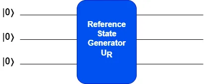
A reference state is like the initial fixed starting point for our problem in quantum computing. To set up this reference state, we need to use a specific, non-variable quantum operation, which we call $U_R$, at the beginning of our quantum circuit. This operation changes our starting state $|0\rangle$ into our reference state $|\rho\rangle$, as in this equation: $|\rho\rangle = U_R |0\rangle$.
If you already have a good idea or data from a previously found best solution, using that as your starting point can make the variational algorithm find the solution faster.
The simplest kind of reference state we can use is called the default state. This is just the starting state of a quantum circuit with n qubits, represented as $|0\rangle^{\otimes n}$. For the default state, our quantum operation $U_R$ is equivalent to the identity operation, represented as $U_R \equiv I$. Because it’s so simple, the default state is a valid starting point that’s used in many situations.
Classical (Unentangled) starting state
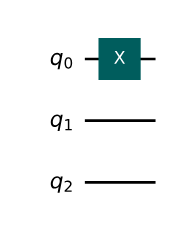
Imagine you have a system with 3 qubits, and you want to start in the state $|001\rangle$ instead of the usual starting state $|000\rangle$. This is an example of what we call a ‘classical reference state’. To create it, you just need to apply a quantum operation called an ‘X gate’ to the first qubit (if we follow Qiskit’s way of ordering qubits). So, we can say $|001\rangle = X_0 |000\rangle$.
In this situation, our quantum operation $U_R$ is equivalent to the X gate applied to the first qubit, represented as $U_R \equiv X_0$. This operation creates our reference state $|\rho\rangle$, which in this case is the same as the state $|001\rangle$.
# Import the QuantumCircuit class from the qiskit library
from qiskit import QuantumCircuit

# Create a new quantum circuit with 3 qubits
qc = QuantumCircuit(3)

# Apply an X gate (also known as a NOT gate) to the first qubit (qubit 0)
# This flips the state of the first qubit: if it was in the state |0>, it becomes |1>, and vice versa
qc.x(0)

# Draw the quantum circuit using matplotlib
# The "mpl" argument tells Qiskit to use matplotlib for drawing
qc.draw("mpl")
Code language: Python (python)
Click here for an explanation of the code above
In this code, a quantum circuit is created with three qubits, all of which start in the state |0>. The X gate is then applied to the first qubit (qubit 0), flipping its state to |1>. The final state of the system is therefore |001>. The `draw(“mpl”)` function is used to visualize the circuit.
Output
Quantum reference state
Let’s say you want to start with a more complicated state that involves both superposition (where a qubit can be in a mixture of states) and entanglement (where qubits are linked so that the state of one directly affects the state of the others). For example, you might want to start with the state $\frac{1}{\sqrt{2}}(|100\rangle+|111\rangle)$.
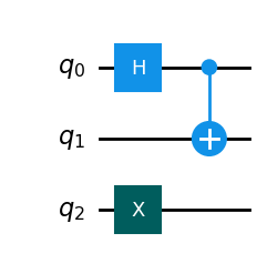
To get to this state from the starting state $|000\rangle$, one method is to use a series of quantum operations. First, apply a Hadamard gate (which creates superposition) to the first qubit, represented as $H_0$. Then, apply a CNOT gate (which creates entanglement) with the first qubit as the control and the third qubit as the target, represented as $CNOT_{01}$. Finally, apply an X gate to the third qubit, represented as $X_2$.
In this case, our quantum operation $U_R$ is equivalent to the sequence of operations $X_2CNOT_{01}H_0$ applied to the starting state $|000\rangle$. This operation creates our reference state $|\rho\rangle$, which in this case is the same as the state $\frac{1}{\sqrt{2}}(|100\rangle+|111\rangle)$.
# Create a new quantum circuit with 3 qubits
qc = QuantumCircuit(3)

# Apply a Hadamard gate to the first qubit (qubit 0)
# The Hadamard gate creates a superposition of states |0> and |1>
qc.h(0)

# Apply a CNOT gate (Controlled-NOT) with the first qubit (qubit 0) as control and the second qubit (qubit 1) as the target
# The CNOT gate creates an entanglement between the control and target qubits
qc.cx(0, 1)

# Apply an X gate (also known as a NOT gate) to the third qubit (qubit 2)
# This flips the state of the third qubit: if it was in the state |0>, it becomes |1>, and vice versa
qc.x(2)

# Draw the quantum circuit using matplotlib
# The "mpl" argument tells Qiskit to use matplotlib for drawing
qc.draw("mpl")
Code language: Python (python)
Click here for an explanation of the code above
In this code, a quantum circuit is created with three qubits, all of which start in the state |0>. The Hadamard gate is applied to the first qubit, creating a superposition of states. Then, a CNOT gate is applied, creating entanglement between the first and second qubits. Finally, the X gate is applied to the third qubit, flipping its state to |1>. The final state of the system is a superposition of |100> and |111>. The `draw(“mpl”)` function is used to visualize the circuit.
Output
Constructing Reference States using template circuits
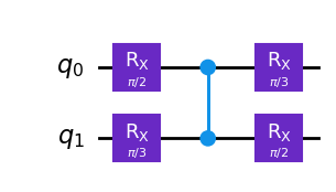
We can also use different template circuits, like ‘TwoLocal’, to make the process of setting up our starting point easier. These templates allow us to easily include multiple adjustable parameters and entanglements. We’ll go into more detail about these template circuits in the next lesson, but for now, know that we can use them for our starting states by setting specific values for the parameters.
# Import the TwoLocal class from the Qiskit library
# This class allows us to create a template circuit with a specific structure
from qiskit.circuit.library import TwoLocal

# Import the math library to get the value of pi
from math import pi

# Create a TwoLocal circuit with 2 qubits, using rotation around X (rx) as the single-qubit gate,
# controlled-Z (cz) as the two-qubit gate, with a linear entanglement structure and 1 repetition of the gate blocks
reference_circuit = TwoLocal(2, "rx", "cz", entanglement="linear", reps=1)

# Create a list of parameter values to be used in the circuit
# Here, we're using specific values of pi for our parameters
theta_list = [pi / 2, pi / 3, pi / 3, pi / 2]

# Bind the parameter values from theta_list to the parameters in the circuit
# This sets the specific values we want for the adjustable parameters in the circuit

reference_circuit = reference_circuit.bind_parameters(theta_list)

# Decompose the circuit into its constituent gates for visualization
# Then draw the circuit using matplotlib
reference_circuit.decompose().draw("mpl")
Code language: PHP (php)
Click here for an explanation of the code above
In this code, a TwoLocal circuit is created with two qubits. The rotation around X (rx) is used as a single-qubit gate and controlled-Z (cz) as a two-qubit gate. The entanglement is linear, and the gate blocks are repeated once. Specific values are set for the adjustable parameters in the circuit, and then the circuit is drawn.
Output
Using Specific Starting States for Quantum Machine Learning
In the field of Quantum Machine Learning, we have something called a Variational Quantum Classifier (VQC). In a VQC, we take our training data and turn it into a quantum state using a special circuit called a ‘feature map’. Each adjustable parameter in this circuit represents a data point from our training set. One type of feature map we can use is the ZZFeatureMap, which allows us to input our data points ($x$ values) into this map.
Here’s the code to do this:
# Import the ZZFeatureMap class from the Qiskit library
# This class allows us to create a feature map that encodes our data into a quantum state
from qiskit.circuit.library import ZZFeatureMap

# Create a list of data points to be used in the feature map
# Here, we're using the values 0.1 and 0.2 for our data points
data = [0.1, 0.2]

# Create a ZZFeatureMap with 2 features (matching the number of data points) and 2 repetitions of the gate blocks
zz_feature_map_reference = ZZFeatureMap(feature_dimension=2, reps=2)

# Bind the data points from the data list to the parameters in the feature map
# This sets the specific values we want for the adjustable parameters in the feature map
zz_feature_map_reference = zz_feature_map_reference.bind_parameters(data)

# Decompose the feature map into its constituent gates for visualization
# Then draw the feature map using matplotlib
zz_feature_map_reference.decompose().draw("mpl")
Code language: Python (python)
Click here for an explanation of the code above
In this code, a ZZFeatureMap is created with two features, corresponding to our two data points. The data points are then set as the adjustable parameters in the feature map. Finally, the feature map is drawn to visualize its structure.
Output

Conclusion
In the realm of quantum computing, setting up an initial state, known as a reference state, is a crucial step for the efficient operation of variational algorithms. These algorithms function similarly to solving a maze – starting at a specific point and then trying different paths until the one that leads to the end is found. The reference state acts as this starting point. There are various ways to construct a reference state, ranging from the simplest default state to more complex states involving superposition and entanglement. The choice of reference state can have a significant impact on how quickly a variational algorithm converges to the best solution.
Creating more complex reference states often involves the use of quantum operations like Hadamard and CNOT gates, or even using template circuits such as TwoLocal, which allows for the expression of multiple tunable parameters and entanglements conveniently. Additionally, in Quantum Machine Learning, a specific type of reference state is used, created with a parameterized circuit known as a feature map. Each parameter value in this feature map represents a data point from the training dataset, effectively encoding the training data into a quantum state for a Variational Quantum Classifier (VQC). This process highlights the versatility and adaptability of reference states in quantum computing, catering to the requirements of different applications and algorithms.
Leave a Reply